ukgeog provides several read_* functions to
provide the ability to easily download official spatial data sets of the
UK as simple feature (sf) objects. A full list of the
geographies available is provided here. Here we demonstrate
how this makes it easy to make choropleth maps with base R, as well as
with popular packages such as ggplot2, tmap
and leaflet.
First we need to read in a spatial dataset as a simple feature
(sf), here we choose to make use of read_admin
to read in the countries that make up the UK:
Note: crs = 4326 (the default) provides the most
compatibility with other functions.
Drawing a choropleth map with a simple feature
We first merge in mid-2019 population density estimates from the ONS, so we have something to plot:
population <- data.frame(
                country = c("England", "Wales", "Scotland", "Northern Ireland"),
                `Population Density` = as.numeric(c("432", "152", "70", "137")),
                check.names = FALSE
              )

sf <- dplyr::left_join(sf, population, by = "country")
Now we plot some choropleth maps with both base R and some easier to use packages:
base R (plot)
cols <- c("#EDF8E9", "#BAE4B3", "#74C476", "#31A354", "#006D2C")
brks <- c(0, 100, 200, 300, 400, 500)
col <- cols[findInterval(sf$`Population Density`, vec = brks)]

plot(sf$geometry, col = col)
legend("bottomleft",
       legend = levels(cut(sf$`Population Density`, brks)),
       fill = cols,
       title = "Population Density")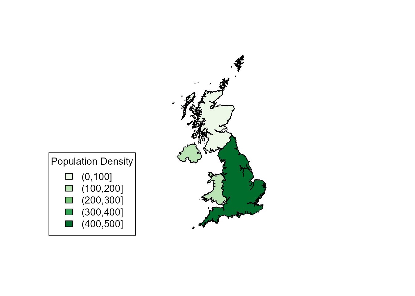
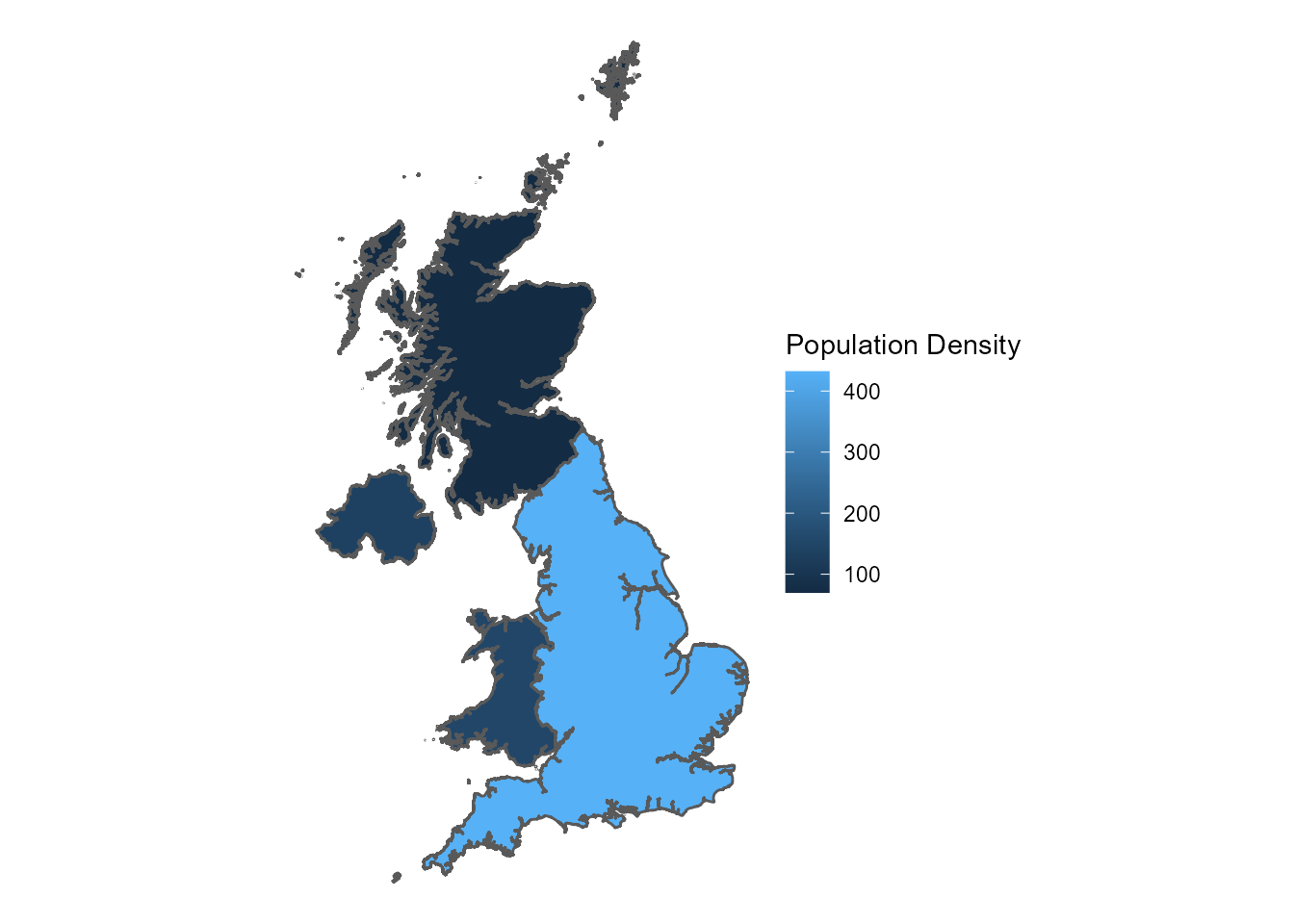
tmap
library(tmap)
#> Warning: package 'tmap' was built under R version 4.1.3

qtm(sf, fill = "Population Density") +
  tm_legend(legend.position = c("left", "top"))
leaflet
library(leaflet)

leaflet(sf) %>%
  addPolygons()